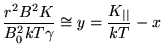
A second solution is possible if one recognizes that the RHS of
equation (9) can be very large as
![]() . In this case we need to expand the exponentials around
. In this case we need to expand the exponentials around
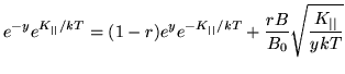
![]() giving,
giving,
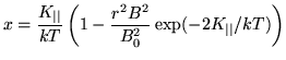 |
(18) | ||
| (19) |
The transition from solution 1 to solution 2 is rather abrupt, since the potential jumps from a few volts to a few kV discontinuously. That is, these are the only two static equilibrium potential solutions, so the intermediate potentials are dynamic, nonequilibrium voltages. One can understand these two states by considering the fate of the cold plasma in these two equilibria. After the initial appearance of hot ions on a particular flux tube, the first eV solution is initially found by the cold plasma, which attempts to shield the hot ions around their density spikes at the mirror point. When the flux tube runs out of cold electrons, occuring first near the equator, the potential rapidly jumps to the second solution as a wave of high space charge potential radiates outward from the equator where the hot ions are ``stripped'' of their shielding electrons.
We call this violation of quasi-neutrality the ``quasi-neutrality
catastrophe'' (QNC). Note that in this second equilibrium the parallel
electric field is opposed to the mirror force, and therefore attempts to
exclude the ions from the equator. Integrating the electric field from the
equator to the mirror point shows that the total potential drop,
![]() , where
, where ![]() is the parallel component
of the kinetic energy at the equator.
In other words, QNC is a transducer converting
parallel hot ion energy into parallel potential, which can be much
larger than the cold electron thermal energy.
is the parallel component
of the kinetic energy at the equator.
In other words, QNC is a transducer converting
parallel hot ion energy into parallel potential, which can be much
larger than the cold electron thermal energy.
![$\displaystyle \frac{r^2 B^2 K}{B^2_0 kT} \cong y [\gamma + 2r-2 +(r-1)^2/\gamma]$](img41.png)